mcmcglm

The mcmcglm package implements the CGGibbs sampler from the article Is Gibbs sampling faster than Hamiltonian Monte Carlo on GLMs?, which has linear run time as a function of number of parameters in a GLM model due to a clever “update” of the linear predictor. See more details at this section in a vignette

The package is implemented in a way that the user can specify any family of the response and any distribution for the prior of the $\beta$ parameter, where $\mathbb{E}[Y|X\beta]=g^{-1}(X\beta)$ for a link function $g$ specified by the family. See more in vignette("pospkg").

Installation

Installation available from GitHub with:

devtools::install_github("mathiaslj/mcmcglm")

Example

We first simulate some data from a linear model to use for showcasing the use of mcmcglm for a gaussian family.

n <- 1000
x1 <- rnorm (n)
x2 <- rbinom (n, 1, .5)
b0 <- 1
b1 <- 1.5
b2 <- 2
lin_pred <- b0+b1*x1+b2*x2

y_norm <- rnorm(n, mean = lin_pred, sd = 1)
dat_norm <- data.frame(Y = y_norm, X1 = x1, X2 = x2)

The use of the function mcmcglm is then similar in interface to the glm function but with an added mandatory specification of

• the prior of the parameter $\beta$
• a tuning parameter for the slice sampling procedure specified by the qslice_fun argument.
  • The default is the qslice::slice_stepping_out function, which performs slice sampling as described in Neal 2003 for which a slice width w needs to be specified.

norm <- mcmcglm(formula = Y ~ .,
                family = "gaussian",
                data = dat_norm,
                beta_prior = distributional::dist_normal(0, 1),
                w = 0.5)

This creates an mcmcglm object which prints as

norm
#> Object of class 'mcmcglm'
#> 
#> Call:  mcmcglm(formula = Y ~ ., family = "gaussian", data = dat_norm, 
#>     beta_prior = distributional::dist_normal(0, 1), w = 0.5)
#> 
#> Average of parameter samples:
#>   (Intercept)       X1       X2
#> 1    1.011134 1.490459 2.026047

summarising the call of the function with averages of the samples of each parameter in the GLM model.

Investigating results

The averages shown in the print method of the object can be retrieved with the generic coef like so:

coef(norm)
#>   (Intercept)       X1       X2
#> 1    1.011134 1.490459 2.026047

Quantiles of the samples (that are not marked as burnin) are available with the quantiles() method, which as a default has probs = c(0.025, 0.5, 0.975):

quantile(norm)
#>           var     mean    q_0025     q_05   q_0975
#> 1 (Intercept) 1.014583 0.8349995 1.013909 1.099346
#> 2          X1 1.457432 0.6940698 1.497910 1.569321
#> 3          X2 1.996584 1.8807500 2.024372 2.177676

The full data set of samples can be accessed with the samples function:

head(samples(norm))
#>   (Intercept)           X1          X2 iteration burnin
#> 1   0.6173367 -0.004541141 -0.09125636         0   TRUE
#> 2   2.6508146  0.281295470  0.68343132         1   TRUE
#> 3   0.8240996  0.324627659  2.30889073         2   TRUE
#> 4   0.8170086  1.028326905  2.20351455         3   TRUE
#> 5   0.8777350  1.592074284  2.16115289         4   TRUE
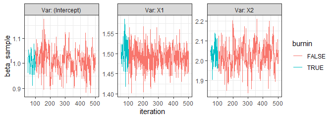
#> 6   0.9092187  1.442872350  2.02913214         5   TRUE

A trace plot can be seen with the function trace_plot:

trace_plot(norm)